Based on Coursera ‘NLP Specialisation’. deep learning.ai
This first course (out of 4) teaches about classification and vector spaces. Classifying pieces of the text into positive sentiments and negative sentiments. That will be done with the help of traditional machine learning methods such are logistic regression and naive Bayes classifiers. Moreover in this course word, text embeddings are covered. That will be helpful further to build machine translation systems. In addition, an efficient tool for searching, locality sensitive hashing method is also taught.
Positive and negative sentiment .
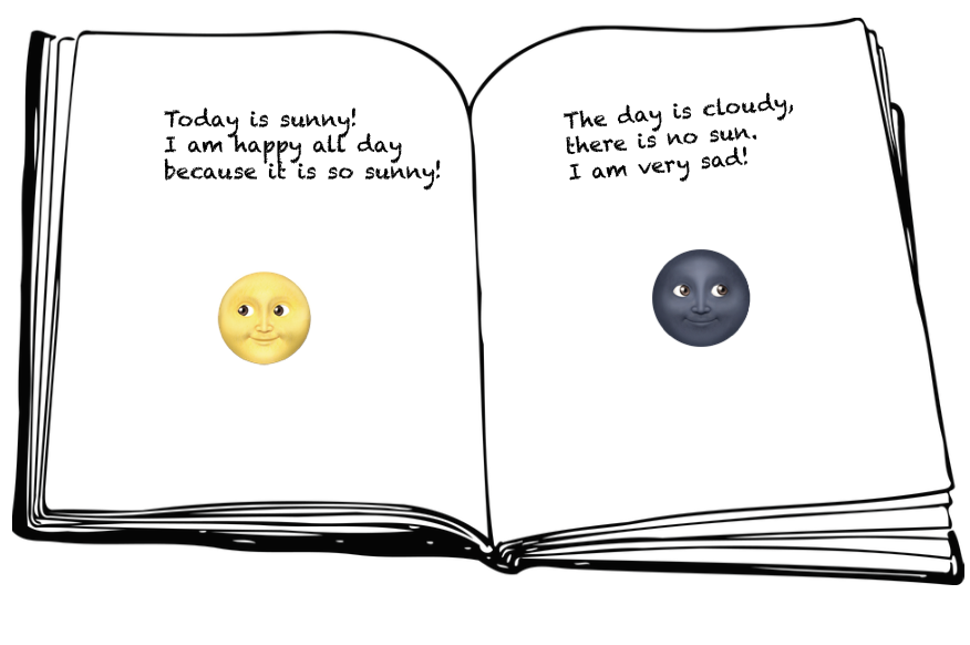
Sentiment analysis helps us to classify texts, sentences, phrases into categories, depending on the sentiment they carry. For instance, on the below pages, the first page carries positive sentiment. How we figured it out? Well, by only looking at the words such as happy, sunny is not enough. The counterexample to it is the sentence: “I am not happy as it is too sunny”. Here we also see word happy and sunny. However we also see a new word not. On the second page we see that sentiment is negative as somebody is not happy without the sun. The words such us cloudy, sad can give us a clue, although we can see the word sun. Sentiment analysis can be tricky, for example, sarcasm, jokes are even hard to fully understand by people. But we can built initial simple models that will try their best and give even not a bad results in sentiment analysis.
First we collect our sentences with labels. Label 1, stands for sentences carrying positive sentiment and 0 for negative. (We will not for now consider ambiguous sentences which partially sad/happy and etc).
Learning on the data with all given labels is called supervised Machine Learning. We will use simple Logistic regression for our classification task. The task is simply to classify into two categories 0 or 1.
But first let’s prepare the data.
Vocabulary
The simple way to represent the data is to encode it into some numerical form (crucial for ML algorithms).For that we will define Vocabulary. Vocabulary consists of unique words in all our data. Define V as the size of the vocabulary. If we had as Vocabulary only those sentences in the picture of the book above, the vocabulary consisted of words:
today, is, sunny, I, am, happy, all, day, because, it, so, sunny, the, cloudy, there, no, sun, very, sad. V = 19.
Then each sentence we will represent as the vector of dimension V. And that vector will consist of 0 and 1. 1 will be placed if the sentence has the corresponding word. For example, first sentence: Today is sunny. [1 1 1 0 …0] according to the vocabulary and corresponding indices. It just happened that we put the words today, is, sunny into 0,1, 2, indices. (Python indices start with 0). And another example:The day is cloudy. Where corresponding vector will look like [0 1.. 1 .. 0 .. 1 1 0 ..] where where indices of 1, 7, 13, 14 are 1 and others are 0.However if we have vocabulary of million words and holding each vector in the memory .. it will be heavy. So maybe we will look at better ways in encoding the sentences.
Feature Extraction with Frequencies.
Let’s also now do something different.Given a particular word, try to see how many time it appears in positive sentiment sentences of negative sentences. We can already conclude that word happy would be in positive class more often. (However it is not always true for a small corpus).So we construct the table with all the words (vocabulary) and corresponding counts in Positive sentences and count in Negative sentences.It should look like this:
| Vocabulary | PosFreq() | NegFreq() |
| today | 1 | 0 |
| is | 2 | 2 |
| sunny | 1 | 0 |
| I | 1 | 1 |
| am | 1 | 1 |
| happy | 1 | 0 |
| all | 1 | 0 |
| day | 1 | 1 |
| because | 1 | 0 |
| it | 1 | 0 |
| so | 1 | 0 |
| …. |
(If you spot a mistake please write it in comments)
So we see that some words appear only in PosFreq() some in NegFreq(). However as was mentioned above it is not a feature of a robust sentiment analyzer.But we can also see that words as I, day, is, am do not carry any meaning. Towards the sentiment . They can be equally in both sentences. Often when analysing complex texts such words are removed as the features as they do not have an influence on the final output.
Now we can construct a feature for the entire sentence. Using the table above, we can calculate look at all words which are in the sentences and then calculate the overall positive and negative frequencies. Take for example and look at the table:
Today is sunny . Today has 1 for PosFreq() and 0 for NegFreq(). is (2, 2) and sunny (1, 0). We sum all PosFreq() that are 1(today) + 2(is) + 1(sunny) = 5. And for NegFreq() is 0+2+0 = 2.So we have (5, 2). We will also add third component which is a bias component. For now it is 1. In general the vector representation for Today is sunny looks like (1, 5, 1).
